Recent Advancements in Russian Roulette and Splitting for Monte Carlo Light Simulation
This post is a re-write of the directed research completed during my masters at USC in spring 2023, reviewing techniques in Russian roulette & splitting and detailing the development of a unidirectional forward path tracer demonstrating recent advancements. This version condenses the series into the key technical elements - if you’d like to read the original series you can find the first post here: Albedo to EARS, Pt. 1. If you find any errors, please leave a note in the comments at the bottom of the page.
Source code is available on GitHub here: roblesch/roulette
Table of Contents
- Introduction
- Core Renderer Architecture
- Literature Review
- Implementing ADRRS and EARS
- Results
- References & Resources
Introduction
In fall 2022 I submitted a project proposal for a directed research project in the following spring. The goal of the project was to implement a path tracer demonstrating landmark techniques in Russian roulette, from the simple albedo-based techniques of the early 90’s to the AI-denoiser-augmented “EARS” recently published at SIGGRAPH ‘22. The proposal was accepted, and over the semester I implemented the path tracer while sharing the development series as a bi-weekly development blog.
Path tracing is a computer graphics Monte Carlo method for rendering three-dimensional scenes by simulating the paths of light particles and their interaction with media as they travel from a light source to an observer. Path tracing is an offline rendering technique utilized for its ability to produce high-fidelity and physically-plausible images. Russian roulette and splitting augment path tracing by eliminating paths that are unlikely to make a significant contribution to the final image (roulette/culling), and branching paths in regions of high importance (splitting). Weights proportional to the probability of culling or splitting are applied to the resulting path value to prevent bias.
Efficiency aware Russian-Roulette and Splitting, or EARS, is a technique presented in a publication by Alexander Rath and others at the University of Saarland submitted to SIGGRAPH in 2022. It enhances previous techniques in Russian roulette and splitting by Vorba and Křivánek by iteratively selecting Russian roulette and splitting parameters such that an efficiency estimate is optimized. By optimizing with respect to efficiency, EARS is able to spend more of the computation budget in regions with high complexity where the current estimate has a high relative variance, and less in regions where the current estimate approaches convergence.
Core Renderer Architecture
I spent my 2022 winter break laying the groundwork for the path tracer that would implement EARS. Based on observations from previous projects, the path tracer was designed with the following in mind:
- Consume public assets. Making scenes from scratch or in code is overly tedious.
- Straightforward and easily debuggable. Debugging numerical issues becomes more difficult as the number of abstraction increase. Performance isn’t critical.
- Extensible. Base classes should have enough modularity to support all the functionality for EARS.
With these values in mind, I evaluated some popular open-source offline renderers as references.
Reference Renderers
Mitsuba3
Popular in the research community, Mitsuba3 is a highly cited renderer supporting a broad variety of techniques, materials and integrators. Its XML-based scene format is easy to parse, and various test scenes are available. With the use of Dr.Jit, many of the core mathematical operations are fairly abstracted, and Dr.Jit’s documentation is difficult to navigate.
Pbrt-v3
Pbrt-v3 is the accompanying source code for the popular “Physically Based Rendering - From Theory to Implementation”. PBRT offers a rigorous discussion of state-of-the-art path tracing techniques, and like Mitsuba, has many test scenes publicly available. Ingo Wald’s PBRT parser can help with scene digestion. The pbrt source is more in the style of a production renderer and well documented.
Tungsten
The top choice for this project, Benedikt Bitterli’s Tungsten checks all the boxes. Its scenes are encoded in an easy to parse JSON format, and its implementations are straightforward and easy to understand. The only hiccup here is that the code is a bit out of date, and needs to be debugged in VS2013. There is a set of test scenes aviailable on Benedikt’s personal site. Tungsten is the primary reference for this project, and the core path tracing algorithm is adapted directly.
Other Dependencies
Architecture
1
2
3
4
5
6
7
8
9
10
11
12
13
14
15
16
17
18
19
20
21
22
23
24
25
┌────────┐
│Renderer│
└───┬────┘
    │
    │ ┌───────────┐
    ├─┤FrameBuffer│
    │ └───────────┘
    │ ┌──────────┐
    ├─┤Integrator│
    │ └──────────┘
    │ ┌─────┐
    └─┤Scene│
      └──┬──┘
         │ ┌──────┐
         ├─┤Camera│       ┌─────┐
         │ └──────┘     ┌─┤Shape│
         │ ┌──────────┐ │ └─────┘
         ├─┤Primitives├─┤
         │ └──────────┘ │ ┌────────┐
         │ ┌─────────┐  └─┤Material│
         ├─┤Materials│    └────────┘
         │ └─────────┘
         │ ┌──────┐
         └─┤Lights│
           └──────┘
The Renderer class is the parent that encapsulates all renderer state, configurations, and scene information. The FrameBuffer is the per-pixel color accumulator where path results are stored. The Scene encapsulates all scene state - the Camera, Materials, Lights and Primitives. Primitives are visible scene geometry that have a Shape, a transform (position, rotation, scale), and a Material. Smart pointers are utilized extensively to prevent duplication of assets in memory. The Integrator performs path tracing on the Scene and stores results in the FrameBuffer.
There’s a lot more to the renderer than this - especially once EARS is integrated - but these are the main pieces. If you want all the gory details, check out the source.
Core Implementation & Debugging
With the architecture in mind and skeletal classes bootstrapped, the first pass of implementation was a DebugIntegrator. As the name suggests, it’s a trivial implementation of the Integrator that maps pixel coordinates to RGB values.

Primitives
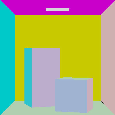
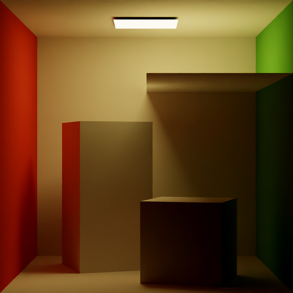
The next goal was to render the “Cornell Box” scene provided on Benedikt’s Rendering Resources page. This scene is the ray tracing “hello world” that makes it easy to demonstrate various effects with minimal primitives. In this case, the only primitives required to intersect the scene are Rectangle and Cube.
A rectangle is a unit square in the XZ plane with a linear transform to the world coordinate system. Intersections are calculated by transforming an intersecting ray into the rectangle’s model space, intersecting it with the XZ plane, and checking if the intersection lies within the base and edges.
Reference implementation: tungsten/Quad.cpp
A cube is a unit cube centered on the origin with vertices at (-1,-1,-1) and (1,1,1). Intersections are calculated by transforming an itnersecting ray into the cube’s model space, checking the ray’s intersections with each of the XY, YZ, XZ planes, and seeing which is the nearest intersection that lies within the cube’s boundaries.
Reference implementation: tungsten/Cube.cpp
Normals
Primitives have constant normals tangent to the face of the surface. As such, no interpolation or uv mapping is required - for a rectangle, simply transform the unit positive normal to the XZ plane to world coordinates. For the cube, find which face is closest to the point of intersection and transform that face’s unit normal to the world coordinates.
A simple NormalIntegrator can be implemented that shoots rays into the scene, intersecting with the primitives and returning the surface normal as an RGB value.
Materials
The Cornell Box scene uses only simple Lambertian BSDFs. References widely available, I referenced description in pbrt and Tungsten’s LambertBSDF.
Lights are represented as primitives with an Emitter, that emit the light’s radiance.
Path Trace Integrator
Now that the primitives are defined, Tungsten’s core path tracing loop can be grafted onto this project. I found it helpful to begin with some review of path tracing fundamentals.
Some useful materials:
- Philip Dutré’s Global Illumination Compendium
- PBRT’s chapter on Monte Carlo Integration
Implementation was grafted from tungsten/PathTracer.cpp and tungsten/TraceBase.cpp. My implementation is available at roulette/pathtracer.cpp.
After the first pass, these were the results at 1 sample per pixel:
Not quite right. Many of the pixels show far too much variance; the light should be consistently white, and there shouldn’t be as many bright spots in dark areas. After some debugging, the following changes produced the correct result:
A. Material references were not properly cleared between intersections.
B. Light was emitting from both sides of the plane.
C. Paths traveling from diffuse surfaces directly to the light oversampled the light.
Great! With the base path tracing algorithm working correctly, I could turn my attention to a deeper review of EARS and related techniques.
Literature Review
Before discussing any one particular technique, there are some unifying concepts to highlight.
- Monte Carlo estimators are shown to converge given a sufficient quantity samples from unbiased estimators.
- Bias is the difference between an estimator’s expected value and the true value of the estimated parameter.
- Variance, \(\sigma^2\), is the measure of the difference between some sample and the true value of the sampled property, generally discussed per-pixel here.
- Efficiency, \(\epsilon = \frac{1}{\sigma^2\tau}\), is the inverse product of variance and computational cost. As variance or cost are reduced, efficiency increases.
Particle Transport and Image Synthesis, Arvo & Kirk 1990
Arvo & Kirk’s 1990 publication was the first to adapt the Particle Transport technique of Russian Roulette to the Light Transport problem. They propose a simple algorithm:
1
2
3
4
5
6
if weight < Thresh then
    begin
    sample s uniformly from [0, 1]
    if s < P then terminate path
    else weight = weight/(1-P)
    end
At some intersection along some path, with termination probability \(P\), further path construction is terminated if some random uniform sample is less than \(P\). Critically, Arvo & Kirk demonstrate that their formulation of Russian Roulette does not introduce bias into the estimator by demonstrating that the expected value of the estimator, \(E(W)\) with original expected value \(\mathcal{w}\), remains unchanged -
\[E(W) = P(termination) * 0 + P(survival) * \frac{\mathcal{w}}{1-P} = P*0 + (1-P)*\frac{\mathcal{w}}{1-P} = \mathcal{w}\]Arvo & Kirk also propose using a material’s albedo (color) for \(P\). This follows physical properties - darker materials appear darker to the human eye because they reflect less light.
They also introduce the concept of splitting, where one path is split into many, increasing the total number of samples. Intuitively and by definition of the Monte Carlo algorithm, increasing the number of samples will reduce variance. So, by combination of Russian Roulette and Splitting (RRS), a net reduction of variance at the same or less net computational cost can result in an increase in efficiency.
Adjoint-Driven Russian Roulette and Splitting in Light Transport Simulation, Vorba & Křivánek 2016
Fast forward some time to 2016 and Russian roulette & splitting have become standard techniques in light transport simulation. Vorba & Křivánek observe that choosing RRS probabilities from local properties such as albedo or throughput do not perform well in scenes with non-uniform light distribution, e.g. diffuse scenes indirectly lit by a powerful occluded light, or in scenes with many dark surfaces which will cull too many paths.
They propose two techniques to address these shortcomings, Adjoint-Driven Russian Roulette & Splitting (ADRRS) and the Weight Window.
ADRRS evaluates the RR/splitting factor \(q\) as the ratio between the total expected contribution of some particle to the expected pixel value I.
\[q(y,\omega_i) = \frac{E[c(y, \omega_i)]}{I} = \frac{v_i(y,\omega_i)\Psi_o^r(y,\omega_i)}{I}\]Where total expected contribution \(E[c(y, \omega_i)]\) is the product of the path weight \(v_i(y,\omega_i)\) at point \(y\) from direction \(\omega_i\) and the reflected adjoint quantity \(\Psi_o^r\). The adjoint quantity estimate \(\tilde{\Psi_o^r}\) is cached by pre-computation of a spatial distribution which approximates irradiance and diffuse visual importance building on author’s previous work, On-line Learning of Parametric Mixture Models for Light Transport Simulation, Vorba et al., 2014. The measurement estimate \(\tilde{I}\) is approximated from the adjoint cache using 4 samples per pixel where the cache is queried immediately for diffuse and glossy surfaces (path depth of 1) and continuing on purely specular surfaces.
The weight window applies the splitting factor \(q\) to calculate an interval of acceptable particle weights, \(\langle\delta^-,\delta^+\rangle\) where paths with a weight above the interval are split, and paths with a weight below the interval are terminated.
The weight window is centered on \(C_{WW} = (\delta^- + \delta^+)/2 = \frac{\tilde{I}}{\tilde{\Psi}_o^r(y,\omega_i)}\) with \(\delta^- = \frac{2C_{WW}}{1 +s}\) where the ratio parameter \(s\) is experimentally set to 5.
Finally, the authors combine ADRRS with path guiding methods resulting in the following tracing algorithm:
1
2
3
4
5
6
7
8
9
10
11
12
13
14
15
procedure HandleCollision(x, y, w_i, v_i)
  // previous collision x, current collision y,
  // incident direction w_i, particle weight v_i
  contribute(y, w_i, v_i)
  G = spatialCache(y)
  Psi = calcAdjoint(G, x, y, w_i)
  window = calcWwBounds(Psi, I)
  n, v_j = applyWw(v_i, window)
  for j = 1 .. n do
    w_o = sampleDir(y)
    v_o = updateWeight(v_j, w_i, w_o)
    z = intersect(y, w_o)
    HandleCollision(y, z, -w_o, v_o)
  end for
end procedure
ADRRS is an important step towards EARS - it leverages the same octree cache of scene radiance estimates when selecting RRS parameters. So, correctly demonstrating ADRRS can validate the impelementation of the cache.
EARS: Efficiency-Aware Russian Roulette and Splitting, Rath et al. 2022
Rath et al. extend the work of ADRRS with Efficiency-Aware RRS, where the splitting coefficient is evaluated as to optimize efficiency by minimizing the product of variance and cost. The integer-valued splitting coefficient is identified by performing a fixed-point iteration of the root of the products of local variance to expected variance and local cost to expected cost, which is shown to iteratively optimize \(n_i\) converging to the optimal value:
\[n_i(x) = \gamma_S(n_{i-1}(x)) = \sqrt{\frac{V_y(x)}{\mathbb{V}[\langle I;n_{i-1}\rangle]}\frac{\mathbb{E}[c(\langle I;n_{i-1}\rangle)]}{\mathbb{E}[c(\langle H(x)\rangle)\mid x]}}\]The optimal RR probability \(q\) is then similarly identified via fixed-point iteration where the suffix moment \(M_y(x)\) is the squared estimator value given the prefix \(x\):
\[q_{i+1}(x) = \gamma_S(n_{i-1}(x)) = \sqrt{\frac{M_y(x)}{\mathbb{V}[\langle I;n_{i-1}\rangle]}\frac{\mathbb{E}[c(\langle I;n_{i-1}\rangle)]}{\mathbb{E}[c(\langle H(x)\rangle)\mid x]}}\]The splitting and RR factors can be jointly optimized to form Optimal RRS, with the joint fixed-point function:
\[\gamma_{RRS}(s(x)) = \begin{cases} \gamma_S(s(x)) & \text{if } \gamma_S(s(x)) > 1 \\ min\{\gamma_{RR}(s(x)),1\} & \text{otherwise.} \end{cases}\]Yielding a splitting factor if \(\gamma_S(s(x)) > 1\) and a RR probability otherwise.
These techniques are applied to forward path tracing with some modification to accomodate vector-valued RGB triplets - products of local variance with prefix weight is performed component-wise and averaged. Cost is estimated by counting the number of rays traced by the estimator, and RRS factors are clamped to \((0.05, 20)\) to avoid excessive splitting.
Variance is estimated by comparing the current path estimate to a denoised image produced using Intel Open Image Denoise.
Then the resulting rendering algorithm is as follows:
1
2
3
4
5
6
7
8
9
10
11
12
13
14
15
16
17
18
19
20
21
22
23
function Render
  for i = 1 .. n do
    // set global statistics to 0
    V(i), C(i) = 0
    // initialize local statistics
    C(i), E(i), M(i), nb = 0
    while time budget not exhausted do
      for px in image do
        direction x_1 = SampleCamera(px)
        // estimate radiance
        Lr = LrEstimate(x_1, I_px)
        // update cost
        c(i) += 1 + c
        v(i) += relativeVariance(x_1, L_r, I_px)
      N_spp += 1
    // normalize estimates
    C(i), V(i) /= N_px * N_spp
    I = mergeFramesByVariance(I, I_i, V(i))
    I_t = denoise(I)
    // for each block in the spatial octree
    for B in SpatialCache do
      c_b, e_b, m_b /= n_b
      v_b = computeVariance(M_b, E_b)
With the radiance estimation LrEstimate defined as
1
2
3
4
5
6
7
8
9
10
11
12
13
function LrEstimate(x_k, I_px)
  b = SpatialCacheBin(x_k)
  // fixed-point optimization
  n = optimizeRRS(T(x_k), C(i-1), V(i-1))
  n = clamp(n, 0.05, 20)
  // splitting estimate
  for i = 1 .. n do
    x_k+1 = sampleBsdf(x_k)
    c, Lr += LrEstimate(x_k+1, I_px)
    w += weight(Lr, x_k, w_o, w_i)
    accumulateCost(C(i), E(i), M(i))
    n_b += 1
  return c, w
The final image is computed iteratively by optimizing total cost and variance, where cost and variance are evaluated along each path by LrEstimate. EARS extends ADRRS by iteratively denoising the image estimate and using the denoised image as an estimate on the expected result. This allows EARS to further optimize selection of RRS parameters by referring to both the estimated path contribution from the octree cache with the previous iteration’s per-pixel cost and variance.
Implementing ADRRS and EARS
There are three components to EARS - denoising, the spatial cache, and image statistics. Denoising is used to create an image estimate used in the efficiency calculation. The spatial cache stores the estimated reflected radiance \(L_r\) and its estimated cost of calculation. Finally, the image statistics accumulate the per-pixel relative MSE against the image estimate, produced by denoising.
Open Image Denoise
Intel’s Open Image Denoise is a collection of deep learning based denoising filters used in the EARS algorithm for approximating ground truth images. Recall the formulation of the splitting factor:
\[n_i(x) = \gamma_S(n_{i-1}(x)) = \sqrt{\frac{V_y(x)}{\mathbb{V}[\langle I;n_{i-1}\rangle]}\frac{\mathbb{E}[c(\langle I;n_{i-1}\rangle)]}{\mathbb{E}[c(\langle H(x)\rangle)\mid x]}}\]The quantity \(\frac{V_y(x)}{\mathbb{V}[\langle I;n_{i-1}\rangle]}\) estimates the local variance for some sample \(V_y(x)\) in relation to the “ground-truth” variance \(\mathbb{V}[\langle I;n_{i-1}\rangle]\). Rather than provide a final ground-truth image as input, EARS uses OIDN to iteratively approximate ground truth when evaluating local variance.
The OIDN repository has an excellent overview on the project with snippets and samples. Check it out if you’re curious!
OIDN Setup
The easiest way to get OIDN and its dependencies is by installing the oneAPI Rendering Toolkit. It can also be built from source by including the repository and pulling the training weights from git lfs, but the installer meets all my needs for now.
CMake needs to know where to find OIDN. The oneAPI OIDN Sample Project has a snippet that solves this -
1
2
3
4
5
6
7
8
9
10
11
12
13
14
15
16
17
18
19
20
21
22
23
set(ONEAPI_ROOT "")
if(DEFINED ENV{ONEAPI_ROOT})
  set(ONEAPI_ROOT "$ENV{ONEAPI_ROOT}")
  message(STATUS "ONEAPI_ROOT FROM ENVIRONMENT: ${ONEAPI_ROOT}")
else()
  if(WIN32)
    set(ONEAPI_ROOT "C:/Program Files (x86)/Intel/oneAPI")
  else()
    set(ONEAPI_ROOT /opt/intel/oneapi)
  endif()
  message(STATUS "ONEAPI_ROOT DEFAULT: ${ONEAPI_ROOT}")
endif(DEFINED ENV{ONEAPI_ROOT})
set(OIDN_ROOT ${ONEAPI_ROOT}/oidn/latest)
set(OIDN_INCLUDE_DIR ${OIDN_ROOT}/include)
set(OIDN_LIB_DIR ${OIDN_ROOT}/lib)

find_package(OpenImageDenoise REQUIRED PATHS ${ONEAPI_ROOT})
find_package(TBB REQUIRED PATHS ${ONEAPI_ROOT})

include_directories(${OIDN_INCLUDE_DIR} ${OIDN_ROOT} ${OIDN_GSG_SOURCE_DIR}/src)
link_directories(${OIDN_ROOT}/lib)

target_link_libraries(${APP_NAME} OpenImageDenoise)
I also needed to bundle the dll’s for OIDN and tbb with the executable on Windows. This was simple enough with a couple extra snippets. Where OIDN is resolved, raise the paths to OIDN and tbb binaries:
1
2
3
4
if (WIN32)
    set(OIDN_BIN_DIR ${OIDN_ROOT}/bin PARENT_SCOPE)
    set(TBB_BIN_DIR ${ONEAPI_ROOT}/tbb/latest/redist/intel64/vc14 PARENT_SCOPE)
endif()
Then copy the dlls after building the main executable:
1
2
3
4
5
6
7
8
add_custom_command(TARGET renderer POST_BUILD
    COMMAND ${CMAKE_COMMAND} -E copy_if_different
        "${OIDN_BIN_DIR}/OpenImageDenoise.dll"
        $<TARGET_FILE_DIR:renderer>)
add_custom_command(TARGET renderer POST_BUILD
    COMMAND ${CMAKE_COMMAND} -E copy_if_different
        "${TBB_BIN_DIR}/tbb12.dll"
        $<TARGET_FILE_DIR:renderer>)
On MacOS I had to add the rpath to TBB libs:
1
2
3
4
add_custom_command(TARGET renderer POST_BUILD
    COMMAND ${CMAKE_INSTALL_NAME_TOOL} -add_rpath
        "${TBB_LIB_DIR}"
        $<TARGET_FILE:renderer>)
I was curious if oneAPI would work on Apple Silicon, but it seemed to work fine as long
as I told CMake to target x86.
Once OIDN is available, integrating it into the renderer is straightforward. The OIDN repository has a
snippet for filtering - all I need
to do is provide it with buffers holding the albedo, normals and estimated color of
an image, and it will write a denoised version to an output buffer. Since FrameBuffer stores pixels
as a contiguous buffer of floats, I could pass these buffers directly to OIDN and didn’t need to write
any reshaping on the input or output.
Very cool! Pretty easy to set up and integrate to the render loop, and I’m surprised how easy it was to get it working on both my desktop and my ARM Macbook.
Exploring OIDN
OIDN produces incredible results, and is blazingly fast. Although an incredible powerful tool, OIDN is not a not a miracle solution to the rendering problem; as a denoiser it still relies on quality inputs. I was interested in seeing what OIDN could do with more complex phenomena like non-atmospheric participating media and caustics. I don’t have nearly enough time to add these materials to my renderer at this exact moment, so I instead slapped OIDN to Tungsten to test OIDN on Benedikt’s volumetric caustic and water caustic scenes.
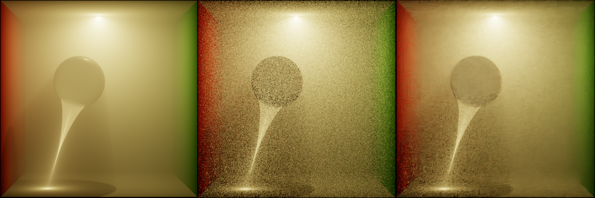
At only 1spp this isn’t the fairest test, but I think it emphasizes the point; without enough information on the input OIDN cannot deduce a physically plausibly denoised output. Visible above, regions with complex caustic phenomena come out of denoising with additional artifacting.
Spatial Cache
With OIDN squared away, the next key component of ADRRS and EARS is the Spatial Cache. The cache bins path estimates for each bounce along the path so that future paths can check the cache to find their nearest estimate and use this estimate as part of the calculation whether to perform russian roulette or split.
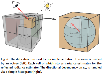
Fortunately, EARS’ author Alexander Rath has some source available on his GitHub that provides reference implementations for both ADRRS and EARS.
Peeking into the source, the octtree.h header seems
to provide everything needed for both ADRRS and EARS. Even better, it only depends on std::array and std::vector.
EARS and Tungsten both implement recursive forward path tracing, and they both use a standard recursive formulation for forward Monte Carlo Light Transport with Multiple Importance:
1
2
3
4
5
Radiance(scene, ray)
    it = scene->intersect(ray)
    Lo += SampleDirectLighting(it)
    Lo += SampleBSDF(it)
    Lo += SampleIndirectLighting(it) // Recursive step
Where they differ is in their termination conditions and how they evaluate shadow rays. Tungsten mixes shadow rays and indirect illumination, and EARS evaluates shadow rays as part of direct lighting. If you’re interested in comparing the two, my implementation of Tungsten’s tracing is available here, and my implementation of EARS’s is here.
With these changes to the tracing algorithm, the next steps to performing ADRRS and EARS are the addition of the spatial cache, filling the spatial cache with the right values, and using those values to compute the splitting factor that determines if a path is terminated (RR) or split (S).
Augmenting tracing with RRS looks something like this -
1
2
3
4
5
6
7
8
9
10
11
12
Radiance(scene, ray)
    it = scene->intersection(ray)
    // 0 : termination, >1 : splitting
    rrs = RRSMethod.evaluate(cacheNode, it)
    // find the bin in the octtree that contains `it`
    node = cacheLookup(its)
    for n = 1 ... rrs do
        Lo += SampleDirectLighting(it)
        Lo += SampleBSDF(it)
        Lo += SampleInderectLighting(it)
        cost += tracingCost
    return cost, Lo
Additionally the integrator is augmented with -
1
2
3
4
5
6
7
8
9
Render(scene, buffer)
    for spp = 1 ... n do
        initializeStatistics(cost, variance)
        for px : buffer
            ray = cameraRay(px)
            Lr, cost, variance = Radiance(scene, ray)
        I = denoise(buffer)
        for block B : cache
            updateVariance(cost, variance)
For each pass over the image, denoising is performed and this estimate of the expected image is used to compute a local variance. The variance and cost are processed in the cache (octtree), and used in each path to produce an RRS value which is 0 if the path should be terminated, and >= 1 if the path should be continued or split.
Image Statistics
The image statistics accumulate the per-pixel relative MSE against the image estimate, produced by denoising. The image statistics performs outlier rejection to prevent especially noisy pixels from overly biasing the estimated variance over the image. These statistics are also used in determining an appropriate RRS value along each path.
Implementation: roulette/imagestatistics.h
Integration & Debugging
With the spatial cache, the tracer, denoising, and image statistics, all the pieces are in place to begin using the EARS algorithm to generate RRS values. The piece that brings all of these steps together is the integrator. The integrator performs multiple iterations over the image, trains the cache, stores variance estimates in the image statistics, performs denoising to produce an image estimate, and merges estimates by variance.
It looks something like this:
1
2
3
4
5
6
7
8
9
10
11
12
13
14
15
16
17
18
19
20
21
EARSIntegrator::render(Scene scene, FrameBuffer frame):
    // render the albedo and normals for denoising
    albedo, normals = renderDenoisingAuxillaries(scene)
    spatialCache = initializeSpatialCache()
    imageStatistics = initializeImageStatistics()
    finalImage = initializeFinalImage()
    foreach iteration in timeBudget:
        rrsMethod = iteration < 3 ? Classic() : EARS()
        iterationImg.clear()
        foreach spp in iterationTimeBudget:
            foreach pixel in image:
                iterationImg.add(earsTracer.trace(pixel))
        // reject variance outliers
        imageStatistics.applyOutlierRejection()
        // train the cache
        spatialCache.rebuild()
        // merge images by variance
        finalImage.add(iterationImg, spp, imageStatistics.avgVariance())
        // produce a denoised estimate
        earsTracer.denoised = OIDN::denoise(iterationImg, albedo, normals)
    frame.result = finalImage.develop()
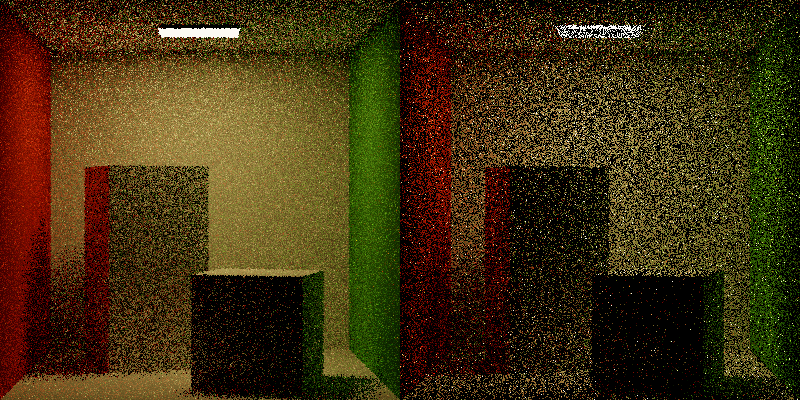
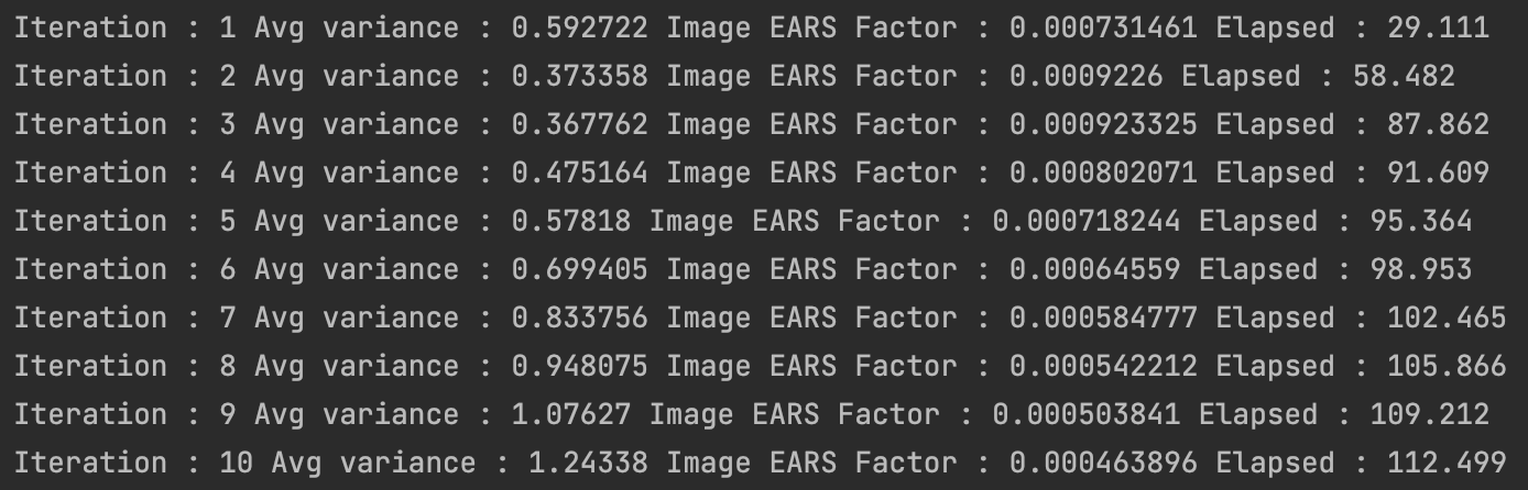
Initial results weren’t quite right. The variance and EARS factor were diverging over each iteration, where they should be converging. There are a handful of sources of error, each of which are quite hard to pin down without solid references to debug against. It could be that the cache is not properly updating or that the values are improperly weighted. Or, the image statistics could have similar issues. Additionally, in the authors implementation image statistics perform outlier rejection per-block rather than per-image-iteration, meaning that more outliers are rejected more frequently.
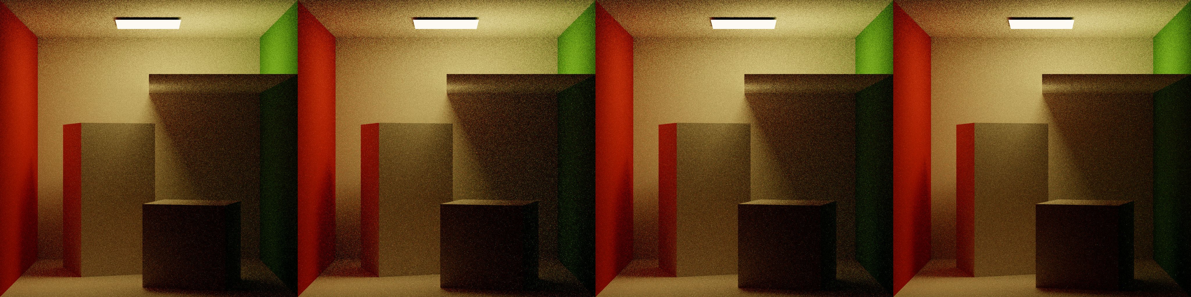
I did a pass on the known issues - the integrator was refactored to render the image in 32x32 blocks and to accumulate image statistics block-wise. I fixed a bug in the tracer where results were being cached even when no samples were collected on that path segment. I updated the scene to add an obscuring panel to create more difficult paths which should make the contributions of ADRRS and EARS more apparent.
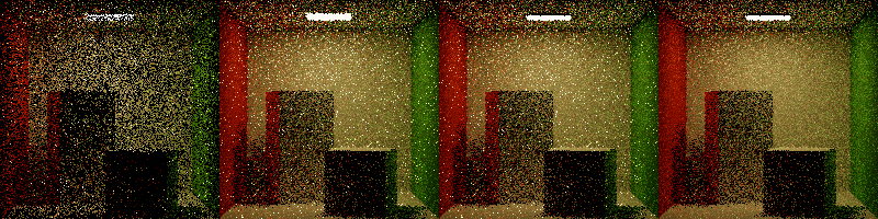
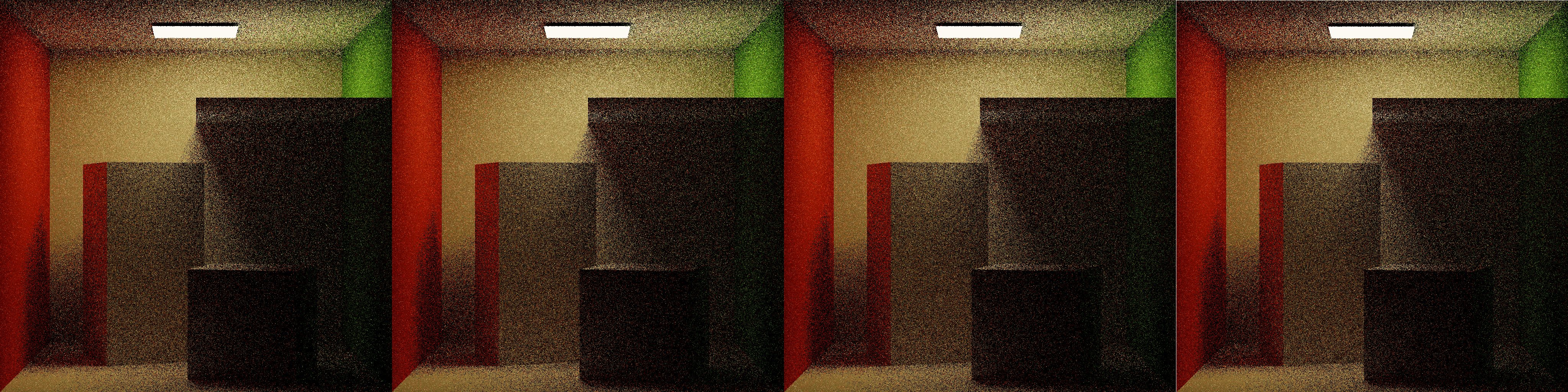
This was an improvement over the above. The leftmost image is the last training iteration, performed with classic RRS. Iterations 4-6 are using EARS. It looked like RRS is no longer diverging quite as aggressively, but it’s still not doing the right thing - the region under the panel should be showing more work performed under EARS via splitting, but it looks like rays are being culled even more often than with classic RRS.
I received a tip from Sebastian Herholz, an engineer at Intel and co-author on EARS. He observed that the RRS was too aggressive and suggested using ADRRS as a means of validating the cache since ADRRS uses only the Lr estimate as its adjoint.
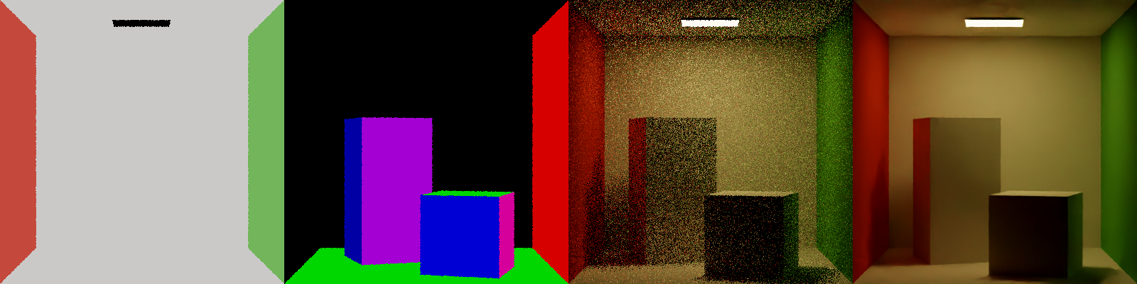
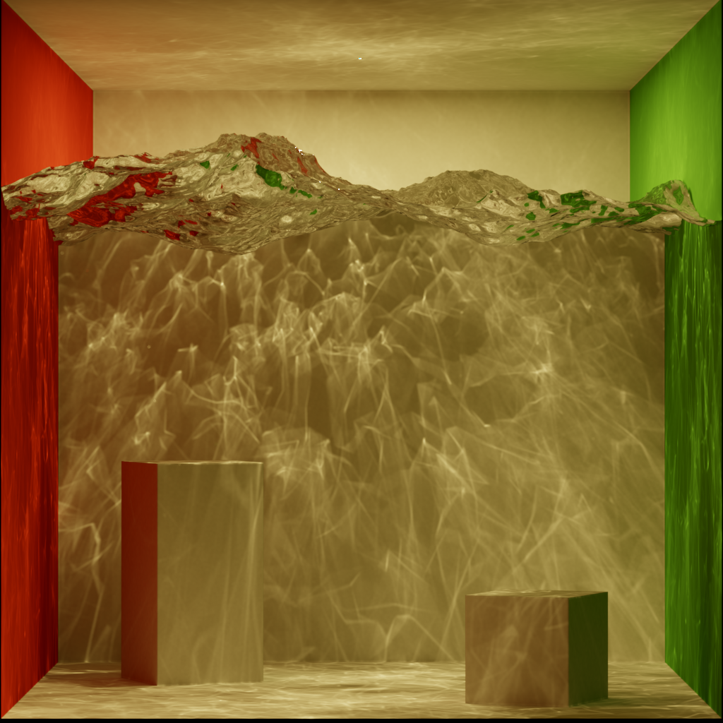
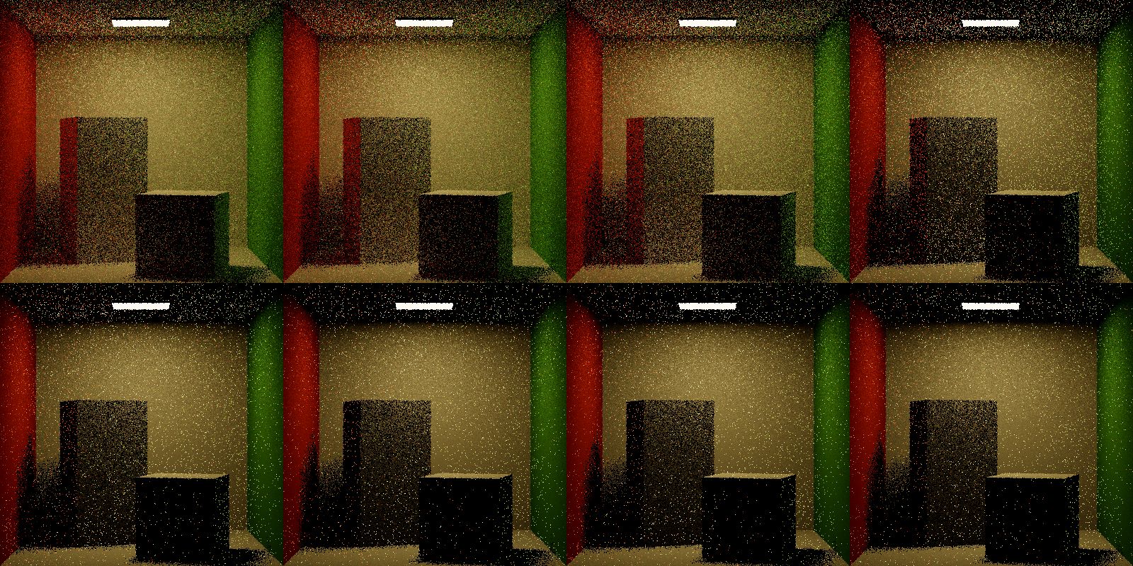
With ADRRS the same issue occurrs - too aggressive RR - but this narrows the issue down to something with the cache. I combed through the cache implementation and found no issues - maybe I was collecting too few samples? I spent quite awhile rendering at higher resolutions, more samples per pixel… quite a painful task in a single-threaded CPU renderer. The number of samples in the cache didn’t seem to have any effect. Maybe I made a mistake in mapping intersections to the cache? After a lot of going in circles, I decided to draw the results of querying the Lr cache. These images are generated by tracing rays into the scene and returning the Lr estimate at the first intersection.
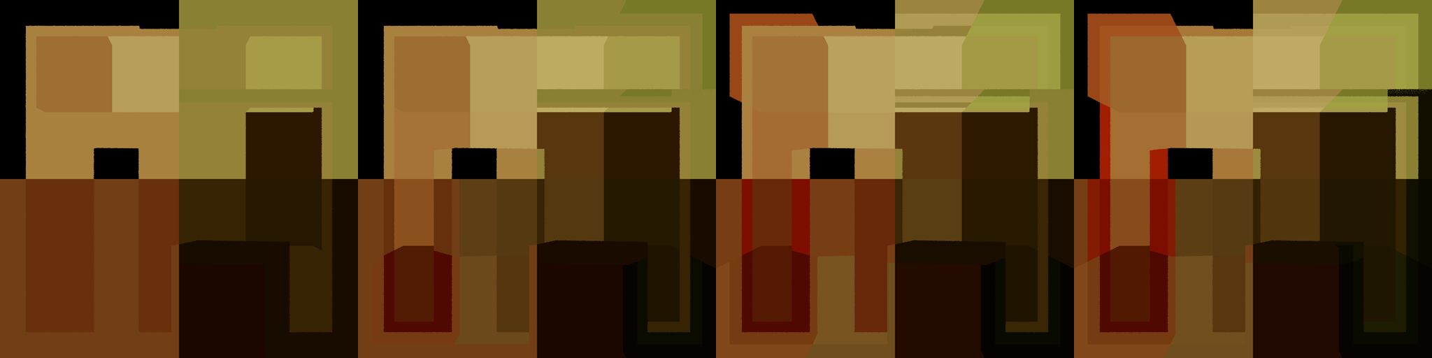
Though not the prettiest thing to look at, it did seem like the cache was doing the right thing. It visibly subdivides over each iteration, correctly maps intersections to the unit cube, and seems to be storing a reasonable approximation of Lr in each bin. Regions in black indicate nodes that haven’t collected enough samples for training, which is appropriately handled in the RR evaluation.
Running out of options, I resorted to combing through the code and comparing it to the original implementation to see if anything was broken or missing. Eventually I found that I was missing this critical piece -
1
2
if (!m_currentRRSMethod.useAbsoluteThroughput)
    input.weight /= pixelEstimate + Spectrum { 1e-2 };
When creating a new primary ray, if the current iteration uses a learning-based method (ADRRS, EARS) the initial weight (throughput) is initialized as the inverse of the current image estimate (denoised merge image over all iterations) plus some normalizing lower-bound. This was the issue all along.
Results
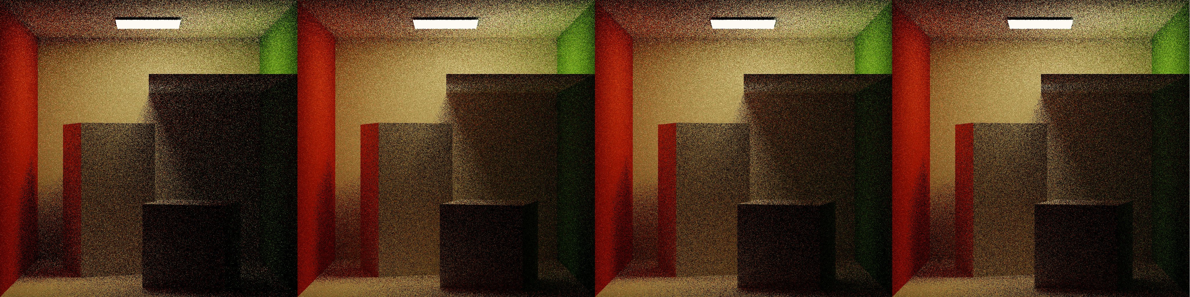
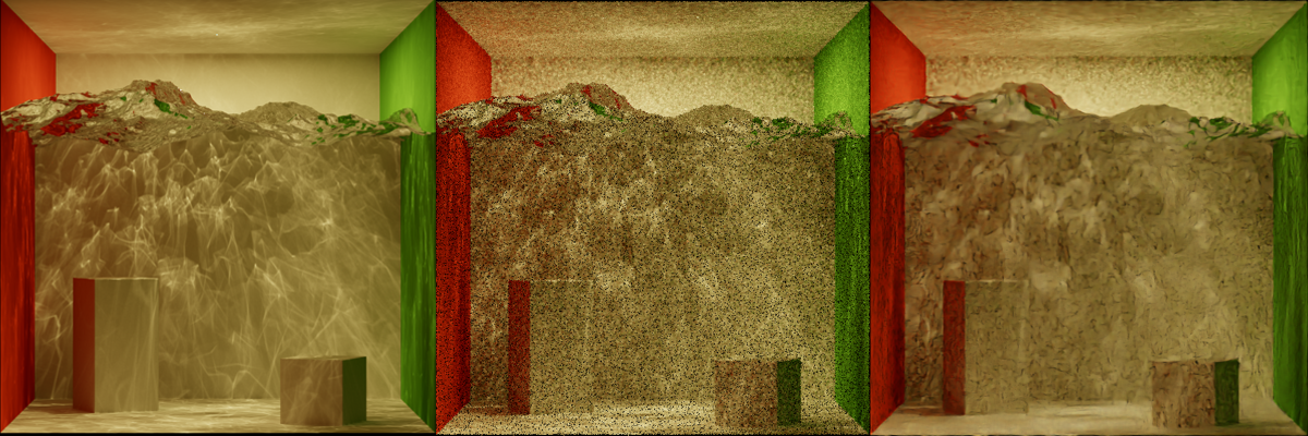
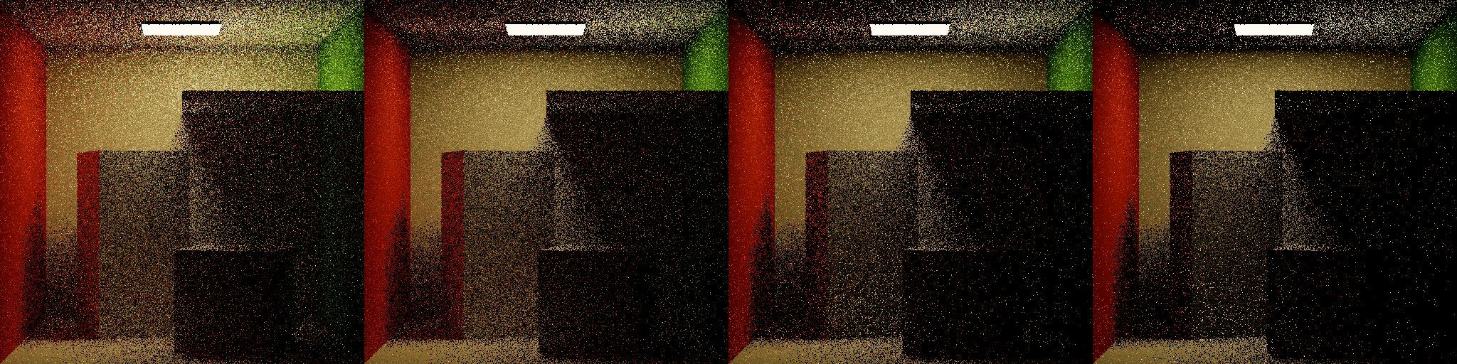
ADRRS and EARS both perform visibly more work in regions with difficult lighting, such as under the panel, and the shadow between the cube and the wall. EARS especially ramps the splitting dramatically in difficult regions before backing off over more iterations.
Shown above are 1 iteration of NoRR, ClassicRR, ADRRS, and EARS, each at 1spp. In ClassicRR, difficult lighting regions are overly punished due to their low throughput. In the same regions under the panel, ADRRS and EARS both emphasize work by performing splitting to gather more information, with EARS creating the most emphasis.
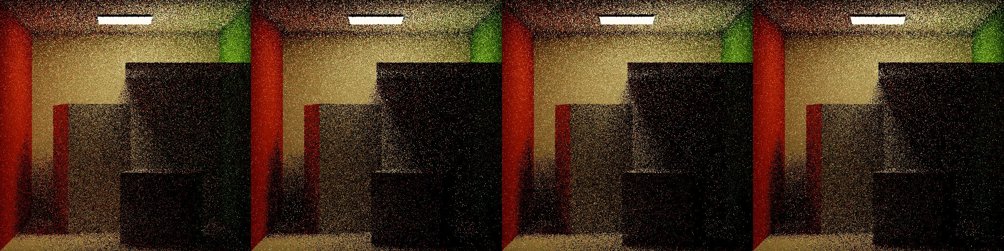
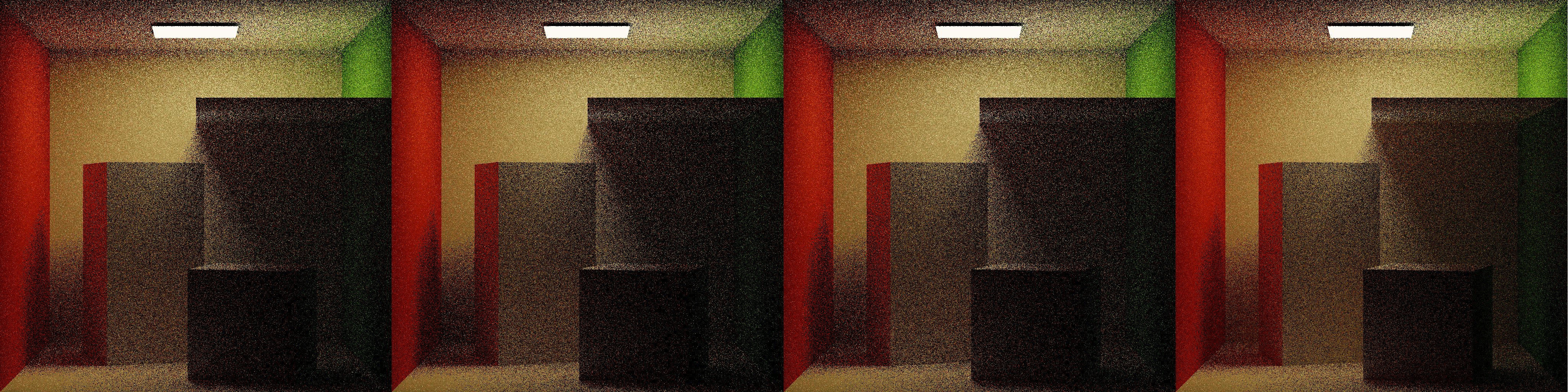
After 16 iterations, ADRRS and EARS both show improvements over NoRR and ClassicRR in the difficult regions under the panel, with EARS showing the greatest improvement.
EARS is a compelling example of integrating a learning-based framework with classic statistical techniques in path tracing. Leveraging deep learning denoising to generate auxiallary inputs to classical RRS demonstrates the power of using trained models to tune values traditionally hand tuned or selected by some hueristic, such as material albedo.
References & Resources
Publications
Matt Pharr, Wenzel Jakob, and Greg Humphreys. 2018. Physically Based Rendering, 3rd edition. https://pbr-book.org/3ed-2018/contents
Eric Veach. 1998. Robust monte carlo methods for light transport simulation. https://dl.acm.org/doi/10.5555/927297
James Arvo and David Kirk. 1990. Particle transport and image synthesis. https://doi.org/10.1145/97880.97886
Jiří Vorba and Jaroslav Křivánek. 2016. Adjoint-driven Russian roulette and splitting in light transport simulation. https://doi.org/10.1145/2897824.2925912
Alexander Rath, Pascal Grittmann, Sebastian Herholz, Philippe Weier, and Philipp Slusallek. 2022. EARS: efficiency-aware russian roulette and splitting. https://doi.org/10.1145/3528223.3530168
Repositories
EARS: Efficiency-Aware Russian Roulette and Splitting. https://github.com/iRath96/ears
Mitsuba Renderer 3. https://github.com/mitsuba-renderer/mitsuba3
pbrt, Version 3. https://github.com/mmp/pbrt-v3
The Tungsten Renderer. https://github.com/tunabrain/tungsten
Intel Open Image Denoise. https://github.com/RenderKit/oidn