Albedo to EARS, Pt. 3 - Into The Thick Of It

Happy Birthday, Nujabes.

This week’s work included some much-needed debugging of the main tracing loop, some extensions for how sampling is conducted, and some rudimentary capability to increase the samples per pixel. I found time to review the literature that provides the project’s foundation, and with that discussion can begin on the interesting part of this project!

Before that, some progress:

Tungsten Uniform Sampling 64 spp, Mine Uniform Sampling 64 spp.

Project proposal: project-proposal.pdf

First post in the series: Directed Research at USC

GitHub repository: roblesch/roulette

Code Updates

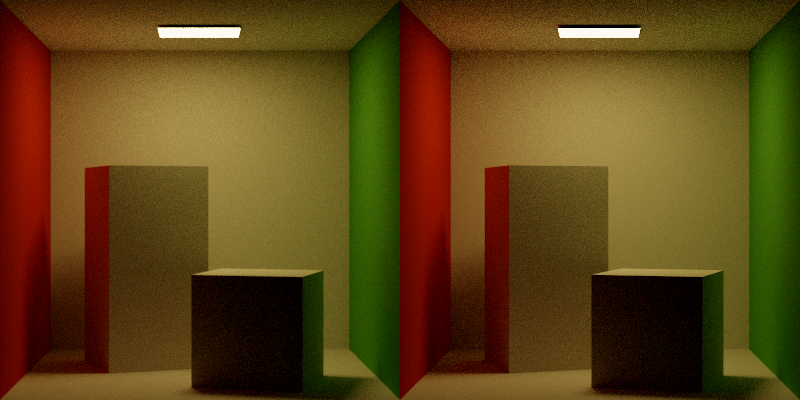
Here’s what changed - the focus over the last two weeks was establishing a stable foundation with the minimum set of behaviors.

Bug Bashing

A. Material references were not properly cleared between intersections.
B. Light was emitting from both sides of the plane.
C. Paths traveling from diffuse surfaces directly to the light oversampled the light.

New Features

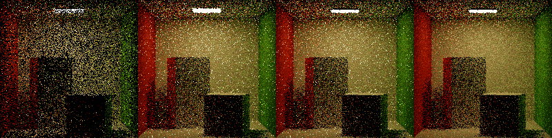
Added a Sampler class for determinably seeded generation of uniform random values
Added a simple accumulation of pixel samples. I’d like to add a reconstruction filter in the future.

With these changes the renderer has a stable foundation for extension with different techniques. Top of my list is some reasonable reconstruction filtering and samplers with better coverage, like a Gaussian Filter and a Halton Sampler. Changes like this are on the back burner pending additional progress on the main goals of demonstrating techniques in Russian Roulette & Splitting. Now some new material!

Reviewing Techniques in Russian Roulette & Splitting

Before discussing any one particular technique, there are some unifying concepts to highlight.

Monte Carlo estimators are shown to converge with enough samples from unbiased estimators.
Bias is the difference between an estimator’s expected value and the true value of the estimated parameter.
Variance \(\sigma^2\) is the measure of the difference between some sample and the true value of the sampled property, generally discussed per-pixel here.
Efficiency \(\epsilon = \frac{1}{\sigma^2\tau}\) is the inverse product of variance and computational cost. As variance or cost are reduced, efficiency increases.

Particle Transport and Image Synthesis, Arvo & Kirk 1990

Arvo & Kirk’s 1990 adapts the Particle Transport technique of Russian Roulette to the Light Transport problem. They propose a simple algorithm:

if weight < Thresh then
    begin
    sample s uniformly from [0, 1]
    if s < P then terminate path
    else weight <- weight/(1-P)
    end

At some intersection along some path, with termination probability \(P\), further path construction is terminated if some random uniform sample is less than \(P\). Critically, Arvo & Kirk demonstrate that their formulation of Russian Roulette does not introduce bias into the estimator by demonstrating that the expected value of the estimator, \(E(W)\) with original expected value \(\mathcal{w}\), remains unchanged -

\[E(W) = P(termination) * 0 + P(survival) * \frac{\mathcal{w}}{1-P} = P*0 + (1-P)*\frac{\mathcal{w}}{1-P} = \mathcal{w}\]

Arvo & Kirk also propose using a material’s albedo or path weight for \(P\).

They also introduce the concept of splitting, where one path is split into many, increasing the total number of samples. Intuitively and by definition of the Monte Carlo algorithm, increasing the number of samples will reduce variance. So, by combination of Russian Roulette and Splitting (RRS), if a net reduction of variance at the same or less net cost can be created, efficiency of the rendering process will increase.

Adjoint-Driven Russian Roulette and Splitting in Light Transport Simulation, Vorba & Křivánek 2016

Fast forward some time to 2016 and Russian Roulette have become standard techniques in Light Transport simulation. As Vorba & Křivánek observe, choosing RRS probabilities from local properties such as albedo or throughput which do not perform well in scenes with non-uniform light distribution, e.g. diffuse scenes indirectly lit by a powerful occluded light, or in scenes with many dark surfaces which will cull too many paths.

They propose two techniques to address these shortcomings, Adjoint-Driven Russian Roulette & Splitting (ADRRS) and the Weight Window.

ADRRS evaluates the RR/splitting factor \(q\) as the ratio between the total expected contribution of some particle to the expected pixel value I.

\[q(y,\omega_i) = \frac{E[c(y, \omega_i)]}{I} = \frac{v_i(y,\omega_i)\Psi_o^r(y,\omega_i)}{I}\]

Where total expected contribution \(E[c(y, \omega_i)]\) is the product of the path weight \(v_i(y,\omega_i)\) at point \(y\) from direction \(\omega_i\) and the reflected adjoint quantity \(\Psi_o^r\). The adjoint quantity estimate \(\tilde{\Psi_o^r}\) by pre-computation of a spatial distribution which approximates irradiance and diffuse visual importance (building on author’s previous work, On-line Learning of Parametric Mixture Models for Light Transport Simulation, Vorba et al., 2014). The measurement estimate \(\tilde{I}\) is approximated from the adjoint cache using 4 samples per pixel where the cache is queried immediately for diffuse and glossy surfaces (path depth of 1) and continuing on purely specular surfaces.

The weight window applies the splitting factor \(q\) to calculate an interval of acceptable particle weights, \(\langle\delta^-,\delta^+\rangle\) where paths with a weight above the interval are split, and paths with a weight below the interval are terminated.

The weight window is centered on \(C_{WW} = (\delta^- + \delta^+)/2 = \frac{\tilde{I}}{\tilde{\Psi}_o^r(y,\omega_i)}\) with \(\delta^- = \frac{2C_{WW}}{1 +s}\) where the ratio parameter \(s\) is experimentally set to 5.

Finally, the authors combine ADRRS with path guiding methods resulting in the following tracing algorithm:

procedure HandleCollision(x, y, w_i, v_i)
  // previous collision x, current collision y,
  // incident direction w_i, particle weight v_i
  contribute(y, w_i, v_i)
  G = spatialCache(y)
  Psi = calcAdjoint(G, x, y, w_i)
  window = calcWwBounds(Psi, I)
  n, v_j = applyWw(v_i, window)
  for j = 1 .. n do
    w_o = sampleDir(y)
    v_o = updateWeight(v_j, w_i, w_o)
    z = intersect(y, w_o)
    HandleCollision(y, z, -w_o, v_o)
  end for
end procedure

EARS: Efficiency-Aware Russian Roulette and Splitting, Rath et al. 2022

Rath et al. extend the work of ADRRS with Efficiency-Aware RRS, where the splitting coefficient is evaluated as to optimize efficiency by minimizing the product of variance and cost. The integer-valued splitting coefficient is identified by performing a fixed-point iteration of the root of the products of local variance to expected variance and local cost to expected cost, which is shown to iteratively optimize \(n_i\) converging to the optimal value:

\[n_i(x) = \gamma_S(n_{i-1}(x)) = \sqrt{\frac{V_y(x)}{\mathbb{V}[\langle I;n_{i-1}\rangle]}\frac{\mathbb{E}[c(\langle I;n_{i-1}\rangle)]}{\mathbb{E}[c(\langle H(x)\rangle)\mid x]}}\]

The optimal RR probability \(q\) is then similarly identified via fixed-point iteration where the suffix moment \(M_y(x)\) is the squared estimator value given the prefix \(x\):

\[q_{i+1}(x) = \gamma_S(n_{i-1}(x)) = \sqrt{\frac{M_y(x)}{\mathbb{V}[\langle I;n_{i-1}\rangle]}\frac{\mathbb{E}[c(\langle I;n_{i-1}\rangle)]}{\mathbb{E}[c(\langle H(x)\rangle)\mid x]}}\]

The splitting and RR factors can be jointly optimized to form Optimal RRS, with the joint fixed-point function:

\[\gamma_{RRS}(s(x)) = \begin{cases} \gamma_S(s(x)) & \text{if } \gamma_S(s(x)) > 1 \\ min\{\gamma_{RR}(s(x)),1\} & \text{otherwise.} \end{cases}\]

Yielding a splitting factor if \(\gamma_S(s(x)) > 1\) and a RR probability otherwise.

These techniques are applied to forward path tracing with some modification to accomodate vector-valued RGB triplets - products of local variance with prefix weight is performed component-wise and averaged. Cost is estimated by counting the number of rays traced by the estimator, and RRS factors are clamped to \((0.05, 20)\) to avoid excessive splitting.

Variance is estimated by comparison to a denoised image produced using Intel Open Image Denoise.

The resulting rendering algorithm is as follows:

function Render
  for i = 1 .. n do
    // set global statistics to 0
    V(i), C(i) = 0
    // initialize local statistics
    C(i), E(i), M(i), nb = 0
    while time budget not exhausted do
      for px in image do
        direction x_1 = SampleCamera(px)
        // estimate radiance
        Lr = LrEstimate(x_1, I_px)
        // update cost
        c(i) += 1 + c
        v(i) += relativeVariance(x_1, L_r, I_px)
      N_spp += 1
    // normalize estimates
    C(i), V(i) /= N_px * N_spp
    I = mergeFramesByVariance(I, I_i, V(i))
    I_t = denoise(I)
    // for each block in the spatial octree
    for B in SpatialCache do
      c_b, e_b, m_b /= n_b
      v_b = computeVariance(M_b, E_b)

With the radiance estimation LrEstimate defined as

function LrEstimate(x_k, I_px)
  b = SpatialCacheBin(x_k)
  // fixed-point optimization
  n = optimizeRRS(T(x_k), C(i-1), V(i-1))
  n = clamp(n, 0.05, 20)
  // splitting estimate
  for i = 1 .. n do
    x_k+1 = sampleBsdf(x_k)
    c, Lr += LrEstimate(x_k+1, I_px)
    w += weight(Lr, x_k, w_o, w_i)
    accumulateCost(C(i), E(i), M(i))
    n_b += 1
  return c, w

The final image is computed iteratively by optimizing total cost and variance, where cost and variance are evaluated along each path by LrEstimate.

Closing Thoughts

I am extremely pleased to be on the other side of laying the foundations for the path tracer and looking forward to implementing these new integration schemes. At a glance, it seems the renderer has all the pieces in place to demonstrate the above techniques, though creating some scenes with more dark surfaces or a stronger occluded light may be useful if there is no apparent difference in result or performance. Additionally, these techniques are meant to demonstrate efficiency at higher/near-production sample rates, so at the least some basic multithreading could save a lot of time in rendering.

Considering the overlap in spatial cache construction, I will evaluate the possibility of implementing one technique that works for both solutions rather than implementing both techniques sited in the original papers. Fortunately ADRRS and EARS both come with supplemental implementations of the techniques provided, so I will likely find some degree of transferability to this project. Finally, I need to evaluate Intel Open Image Denoise to make sure the framework is functional on my platform.